Dijkstra's Algorithm as a Sequence

Graphs are cool. After slogging through sorting arrays in the the Coursera Algorithms I class it is nice to implement algorithms that aren’t built into the standard library. They are also much more real world. For example finding the shortest path in Eve Online from NOL-M9 to every system in Delve (visualized above using D3.js).

NOTE: You can drag the systems to make sure no lines overlap if that is your thing … it is mine.

Two of my favorite quotes from the Joy of Clojure are:

As author Rich Hickey himself proclaimed, any new class in general is itself an island; unusable by any existing code written by anyone, anywhere. – Fogus & Houser

It is better to have 100 functions operate on one data structure than 10 functions on 10 data structures. – Alan Perlis

In Clojure you can’t go wrong with sequences. In a previous post I turned a graph into a sequence after I discovered I was implementing my own sequence functions on top of it. In this post I’m going to do the same thing with Dijkstra’s Algorithm. This continues my trend of being 5 years behind state of the art Clojure blogging.

Protocols

I created a pretty bare bones protocol for graphs this go around. I’m from C# land so of course I added an I in front of Graph. Old habits and all.

(defprotocol IGraph
  (vertices [g])
  (neighbors [g v])
  (add [g v1 v2 c])
  (cost [g v1 v2]))

Dijkstra’s just cares about neighbors and cost. For completeness here is the implementation of a directed and undirected graph.

(defrecord UndirectedGraph [vs]
  IGraph
  (vertices [_] (keys vs))
  (neighbors [_ v] (keys (vs v {})))
  (add [_ v1 v2 c]
       (-> vs
           (assoc-in [v1 v2] c)
           (assoc-in [v2 v1] c)
           (UndirectedGraph.)))
  (cost [_ v1 v2] (get-in vs [v1 v2])))

(defrecord DirectedGraph [vs]
  IGraph
  (vertices [_] (keys vs))
  (neighbors [_ v] (keys (vs v {})))
  (add [_ v1 v2 c]
       (-> vs
           (assoc-in [v1 v2] c)
           (DirectedGraph.)))
  (cost [_ v1 v2] (get-in vs [v1 v2])))

At the end of the day it is still just a map of maps.

graph

{ :s { :v 1, :w 4 }
  :v { :w 2, :t 6 }
  :w { :t 3 } }

This representation can’t handle multiple edges between the same two vertices though. Maybe next time.

Dijkstra’s Algorithm

I’m not good enough to give a thorough explanation of the algorithm but the main idea is that it finds the shortest path from a vertex to every other connected vertex in a graph. It does this by traversing the graph from vertex to vertex always selecting the cheapest cumulative path with each expansion. In order to do this we keep a list of all vertices that have been explored (they already have a shortest path) and all available vertices for exploration along with their cost. So each iteration is simply selecting the cheapest vertex available to explore and adding its neighbors to the list of available exploration vertices.

Since Dijkstra’s expands one vertex at a time I represent the algorithm as a lazy sequence. Again, our two data structures are the explored vertices and the available frontier vertices to select from.

Here is my first stab.

(defn shortest-paths [g start]
  ((fn explore [explored frontier]
     (lazy-seq
       (if (empty? frontier)
         nil
         (let [[v [total-cost previous-vertex]] (apply min-key (comp first second) frontier)
               path (conj (explored previous-vertex []) v)
               explored (assoc explored v path)
               unexplored-neighbors (remove explored (neighbors g v))
               new-frontier (into {} (for [n unexplored-neighbors]
                                       [n [(+ total-cost (cost g v n)) v]]))
               frontier (merge-with (partial min-key first)
                                    (dissoc frontier v)
                                    new-frontier)]
           (cons [v total-cost path]
                 (explore explored frontier))))))
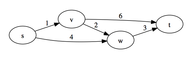
   {} { start [0] }))

Lots going on here so I’ll go through the algorithm line by line with an explanation. I’ll use the following graph which has explored s and is looking to expand.

graph

First thing we do is check if the frontier is empty.

(if (empty? frontier)
 nil
 (let [[v [total-cost previous-vertex]] (apply min-key (comp first second) frontier)

If it is we have explored every connected vertex and can end the sequence by returning nil. If the frontier is not empty we select the vertex with the cheapest cost for expansion. Since we’ve expanded s the frontier would be the following data structure:

{ :v [1 :s]
  :w [4 :s] }

The keys on the map are the available vertices to expand to and the values are a vector of cost and previous vertex. When we apply min-key (comp first second) to frontier we are selecting the map entry with the cheapest cost. (comp first second) transforms [:v [1 :s]] into 1 which would end up being the lowest cost (versus 4 for [:w [4 :s]]). The map entry is then destructured for further use.

Priority Map

One issue with this is that its a linear scan through the frontier. Worst case scenario this could be all vertices which would turn the algorithm into O(n^2). The course recommends the use of a heap data structure for the frontier which would make the algorithm O(n*log(n)). I couldn’t find a clojure persistent heap implementation but there is a persistent priority map which still gets us the logarithmic operations we want.

Finding the cheapest cost path now becomes:

(when-let [[v [total-cost previous-vertex]] (peek frontier)]

We replace the empty? check with a when-let which will return nil if the frontier is empty. peek on the frontier is log(n) and returns the cheapest cost path.

If we benchmark the map version versus priority map version on a graph with ~5000 vertices the algorithm goes from 325ms to 55ms. So thats cool – go data structures! In order to benchmark I used the neato criterium library. It produces a pretty cool little report.

(crit/quick-bench (doall (shortest-paths galaxy 30004712)))

    Evaluation count : 12 in 6 samples of 2 calls.
             Execution time mean : 54.818248 ms
    Execution time std-deviation : 528.273012 µs
   Execution time lower quantile : 54.238498 ms ( 2.5%)
   Execution time upper quantile : 55.504810 ms (97.5%)
                   Overhead used : 2.751427 ns

Now that we’ve selected the cheapest vertex to explore, lets explore it.

; part of the let bindings ...
path (conj (explored previous-vertex []) v)
explored (assoc explored v path)

The explored data structure is a map with the explored vertices as keys and the path to the vertex as a value. The current explored value is { :s [:s] } – we’ve explored :s and the path was just itself. The path to the expansion vertex is the path to the previous vertex conj‘d with the current vertex. We then add it to the explored map. The final result of exploring :v is { :s [:s], :v [:s :v] }.

`merge-with`

Now we need to update the frontier which is a bit more involved. The frontier starts as { :v [1 :s], :w [4 :s] } and we want it to end as { :w [3 :v], :t [7 :v] }. This is from removing :v (its now explored), adding :t as a new vertex from :v with a cost of 7 (1 + 6) and updating :w to be from :v with a cost of 3 (1 + 2) because its cheaper than the existing cost of 4 from :s.

I do this in two logical steps, the first of which is finding all neighbors of the current vertex and their cost.

; part of the let bindings ...
unexplored-neighbors (remove explored (neighbors g v))
new-frontier (into {} (for [n unexplored-neighbors]
                        [n [(+ total-cost (cost g v n)) v]]))

We get the neighbors for the vertex and remove any which are already explored. We then turn it into a map of neighbor to a tuple of cost and previous vertex (which is the current vertex). The end result of new-frontier is { :w [3 :v], :t [7 :v] }.

The next step is to update the existing frontier with these new neighbors. I initially had a complicated one-liner using reduce, update-in and fnil. Then I discovered merge-with which takes multiple maps, merges them together, and resolves duplicate keys with a function you provide. This is awesome. All I need is a function which picks the map entry with the cheapest cost.

; part of the let bindings ...
frontier (merge-with (partial min-key first)
                     (pop frontier)
                     new-frontier)

Here I use (partial min-key first) as the merge function which picks the cheapest cost. I also pop off the cheapest vertex from frontier since we just added it to explored. So merge-with between { :w [4 :s] } and { :w [3 :v], :t [7 :v] } results in { :w [3 :v], :t [7 :v] } which is exactly what we want. merge-with is pretty rad.

So now we have the updated explored and frontier and can recurse.

(cons [v total-cost path]
      (explore explored frontier))

We cons a vector of the current vertex, its total cost, and path to the lazy sequence and then recurse on explore. Voila.

(def G
  (-> (DirectedGraph. {})
      (add :s :v 1)
      (add :s :w 4)
      (add :v :w 2)
      (add :v :t 6)
      (add :w :t 3)))

(shortest-paths G :s)

; => ([:s 0 [:s]] [:v 1 [:s :v]] [:w 3 [:s :v :w]] [:t 6 [:s :v :w :t]])

To `let` or not `let`

So my first take consisted of breaking the algorithm into a bunch of steps using let bindings. I have no idea if this is good or bad. Many of the let bindings are used only once, so for my final solution I removed them. I am left with:

(defn shortest-paths [g start]
  ((fn explore [explored frontier]
     (lazy-seq
       (when-let [[v [total-cost previous-vertex]] (peek frontier)]
         (let [path (conj (explored previous-vertex []) v)]
           (cons [v total-cost path]
                 (explore (assoc explored v path)
                          (merge-with (partial min-key first)
                                      (pop frontier)
                                      (into {} (for [n (remove explored (neighbors g v))]
                                                 [n [(+ total-cost (cost g v n)) v]])))))))))
   {} (pmap/priority-map start [0])))

I think this is way sexier, but I’m worried that I lose some mild amount of documentation the let bindings provide. I don’t know if that is true though. It is one of those things with clojure that you are left with some rather dense code. I wrote this and it would take me awhile to understand what the heck is going on. The flip side is that if I wrote this in C# it would be several times longer and would probably take just as long to figure out as I scroll through code and page between classes.

I guess the take away is to dissociate the amount of code produced and the amount of time to understand. If a little bit of code is doing a lot it is okay for it to take awhile to understanding.

But who knows.

Power of Sequence

So now that I have a sequence it is pretty easy to find the shortest path between two vertices.

(defn shortest-path [g start dest]
  (let [not-destination? (fn [[vertex _]]
                           (not= vertex dest))]
    (-> (shortest-paths g start)
        (->> (drop-while not-destination?))
        first
        (nth 2))))

(shortest-path G :s :t)

; => [:s :v :w :t]

We use the sequence function drop-while to advance the sequence until we find a hit or the sequence ends. I like this. You could follow the same pattern for functions finding cost of paths, the closest N neighbors of a vertex, etc. with each function only expanding the search as much as it needed.

Sequences – not too shabby.